Embedded Devices with Artificial Intelligence:
Keyword Spotting with TinyML and Cortex-M4
Theoretically understood, but not yet practically implemented.
Since we know that challenges often only become visible during actual implementation, we want to reinforce the theory behind AI on embedded systems from our blog post dated March 4, 2025, with a concrete example.
The goal is a “Keyword Spotting” application on a Cortex-M4 microcontroller that demonstrates how AI is finding its way into the embedded world.
You can find the mentioned blog post here: https://www.csa.ch/en/blog/ai-in-embedded-systems-how-it-works
Use Case: “Keyword Spotting”
High-performance devices are often put into standby or sleep mode, partly due to energy requirements prescribed by EU regulations.
During this state, the high-performance processors and internet connection are turned off. A small embedded microcontroller must then be able to wake up the rest of the device without external help. This is known as “Keyword Spotting.”
Famous examples include “Alexa!”, “Okay Google!”, or “Hey Siri.”
To many, this technology may seem trivial, yet it is a prime example of applying a neural network on a platform with very limited resources.
Why is this additional effort necessary?
One key factor is energy consumption. Additionally, data privacy and the protection of personal information play a central role.
Do we want a device that is always listening and analyzing our data?
Wouldn’t we prefer that the service is only activated when we explicitly allow it?
And this is where the “Keyword Spotting” application comes into play. A model specifically trained to detect just a few keywords can be kept compact enough to require almost no computing power or energy—and it works entirely without a permanent internet connection.
The embedded device continuously listens but analyzes only the activation word. All other audio data is immediately discarded.
Additionally, the entire process occurs locally.
The Workflow
This chapter describes the workflow we applied during the course of the project.
1. Defining Design Requirements
This may seem trivial at first. A small device should react to voice input and execute an action when a specific word is identified.
However, further questions arise:
Regarding end-users:
- What language is spoken, and with what accent?
- Is the speech whispered or spoken loudly?
- Should the device respond to only one voice? What happens if my wife or children say the same word?
Regarding deployment location:
- Are we always in a quiet environment, or are there background noises?
- Should the activation word still be detected even in noisy conditions?
- Suppose our device is in the living room, which is usually quiet. What if we open a window and there's a construction site outside?
Regarding data security:
- What happens to the recorded audio data?
- Is it temporarily stored or immediately discarded?
- Is it sent to the cloud for further processing or not?
The list could go on indefinitely. However, it illustrates many aspects that must be considered before getting started.
We will greatly simplify our example, so our requirements are defined as follows:
- The words “Yes” and “No” should be recognized.
- If “Yes” is recognized, a green LED should be activated.
- If “No” is recognized, a red LED should be activated.
- If sounds are recognized but none of the target words, a blue LED should be activated.
- The device will only be used in a quiet environment (office).
- The device should preferably recognize the author’s voice, but will not be personalized or diversified.
- Our device has no internet connection.
- Data will be discarded immediately after processing.
2. Collecting and Preparing Data
Now the data collection begins, which will serve as the foundation for training our model.
This is often the most time-consuming and challenging part. We need a dataset that contains thousands of words and is representative of the intended environment.
While the device is intended to be used “only” in an office setting, there are still background noises to consider.
If these data are to be collected manually, it can be a lengthy and demanding process. We need not only the words “Yes” and “No,” but also as many other words and non-speech audio clips as possible.
This process is greatly simplified by using an existing dataset.
There are several publicly available datasets [1], most of them in English. Since the device is to be trained for “Yes” and “No,” we’ll use a dataset that already contains these words.
A suitable dataset is “speech_commands” by Pete Warden [2].
It contains thousands of recordings for various words, including “Yes” and “No,” which can be used to train our model.
If later personalization (e.g., for a specific voice) is desired, now would be the right time to record your own voice samples and add them to the training dataset.
[1] A list can be found here: https://github.com/jim-schwoebel/voice_datasets
[2] https://arxiv.org/pdf/1804.03209: Speech Commands: A Dataset for Limited-Vocabulary Speech Recognition
2.1 Preparing Audio Data
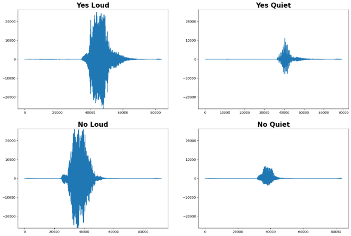
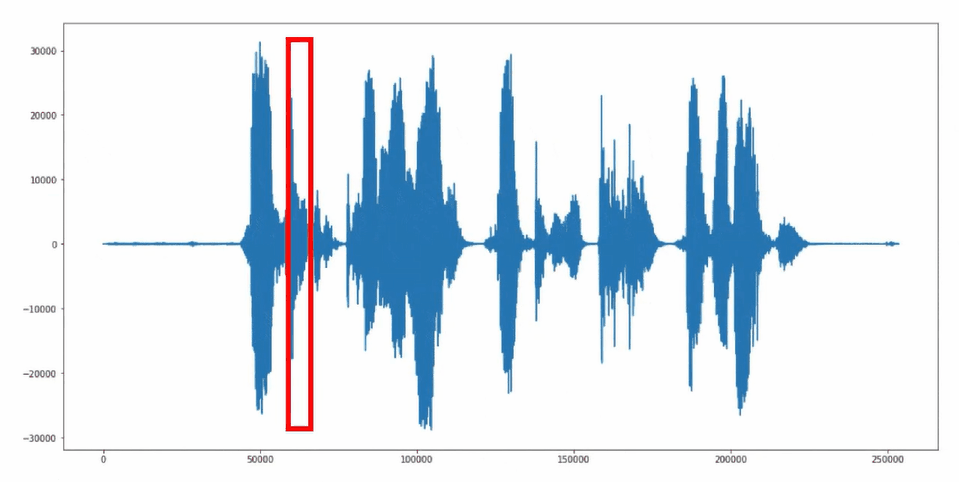
Audio files store the waveform information, which is a discrete-time signal. The model should be able to extract the characteristic features of these signals. However, this is difficult with time-domain signals.
The following image illustrates:
- Same words can look very different
- Different words often look very similar in the time domain
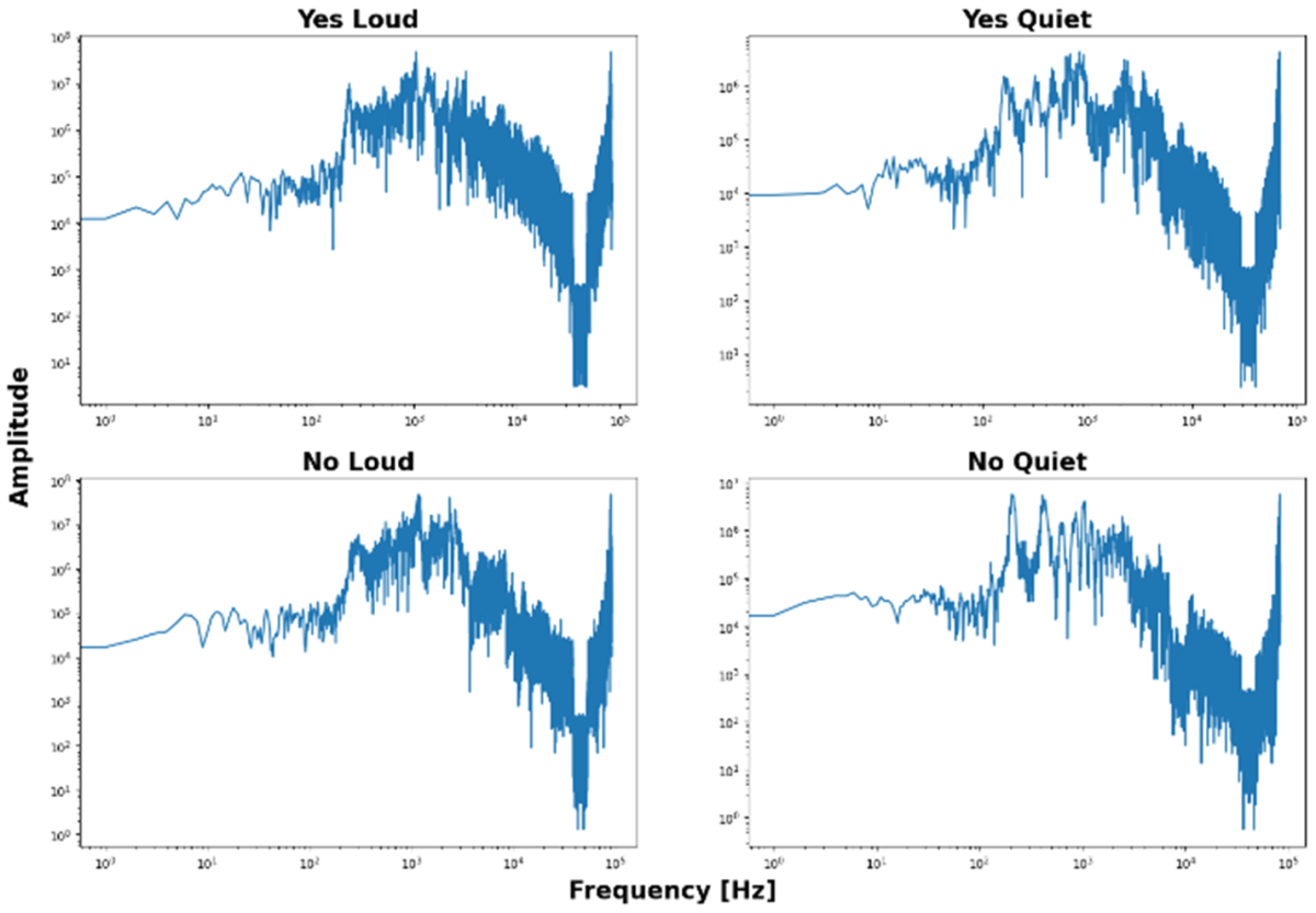
Even a basic conversion to the frequency domain (Fourier transform) doesn’t make the features more distinguishable. While it might reveal pitch or voice timbre, that is insufficient for our application.
The goal is to recognize the **content** of the speech, not the voice or pitch of the speaker.
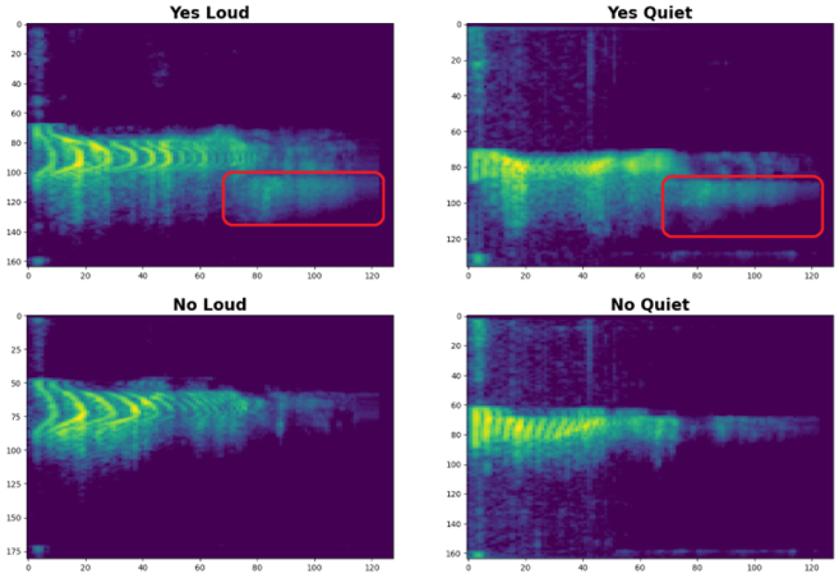
The characteristic features of a word only become visible in the spectrogram, a representation of the frequency spectrum over time.
These similarities can be enhanced further by adjusting the relevant frequency range and increasing the contrast between quiet and loud signals.
Upon closer inspection, we can now clearly distinguish between “Yes” and “No,” regardless of how loudly they are spoken.
While this distinction is obvious to us as humans, an AI model must be specifically trained to reliably detect these differences.
Through this processing, our dataset now becomes a solid foundation for the upcoming model training.
3. Developing and Training the AI Model
We now shift our focus to the neural network. We've already explained how it works and which types of neurons and layers it may contain in the blog post referenced above.
We decided to use TensorFlow.
TensorFlow provides a predefined path for programming embedded devices via TensorFlow Lite and TensorFlow Lite Micro. Alternatives like PyTorch typically require a running operating system, such as iOS, Android, or embedded Linux. TensorFlow doesn’t – it can also be used “bare-metal.”
During the data preparation phase, the audio signals were converted into spectrograms. Therefore, we can apply an existing model that specializes in extracting features from spectrograms or image files.
Even though highly specialized models offer limited functionality, they do so with exceptional efficiency – making them ideal for resource-constrained environments.
3.1 TinyConv
We use the tiny_conv model from TensorFlow.
This consists of four layers, which are sufficient for our embedded application.
- Input Layer
This layer applies the steps mentioned in Chapter 2.1 to convert microphone data into a spectrogram (reshape).
- Convolution Layer
This layer filters the relevant features from the spectrograms.
- Fully Connected Layer (also called Dense Layer)
This layer calculates the probabilities of which word was detected based on the filtered features.
- Output Layer
This final layer classifies the probabilities using the SoftMax activation function.

3.2 Transfer Learning
As established voice assistant technologies suggest, we’re not the first to train such a model. Nor are we the first to use this particular dataset – it was created specifically for such use cases.
There are freely available models that have already been trained on this dataset, saving us days of training time.
We can use a snapshot of such a model as a starting point and continue training from there. TensorFlow allows you to define checkpoints during training, which can later be resumed at any time.
With our specific training data, the model is trained further starting from a checkpoint. A portion of the dataset is reserved for validation. This process results in a final checkpoint that’s suitable for performing inference on a device.
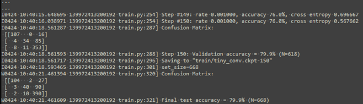
The model achieves an accuracy of around 80%, which is not exceptionally high but could be improved through adjustments in training, model architecture, or training data.
However, doing so would exceed the scope of this test project.
4. Convert, Optimize, and Deploy the Model
The requirements for the model are primarily determined by the hardware on which it will eventually run.
We use a Nordic nRF52480 microcontroller. This Cortex-M4F runs at 64MHz and features 1MB of Flash and 256KB of RAM.
The model therefore needs to be very small to fit on the device. We achieve this by reducing it to only the essential functionalities.
First, we convert the final checkpoint into a model that only performs inference (classification). This process is called "freezing":
In this step, the model is “frozen” at a specific training state.
Further training is no longer possible – but also no longer needed.
4.1 From TensorFlow to TensorFlow Lite
Until now, we’ve been working in the TensorFlow domain – the part of the framework responsible for creating and training the model.
Now we convert the frozen model into a TensorFlow Lite model. In this step, floating-point numbers are quantized to 8-bit integers, among other changes.
The training dataset is also converted accordingly to allow post-conversion testing of the model.
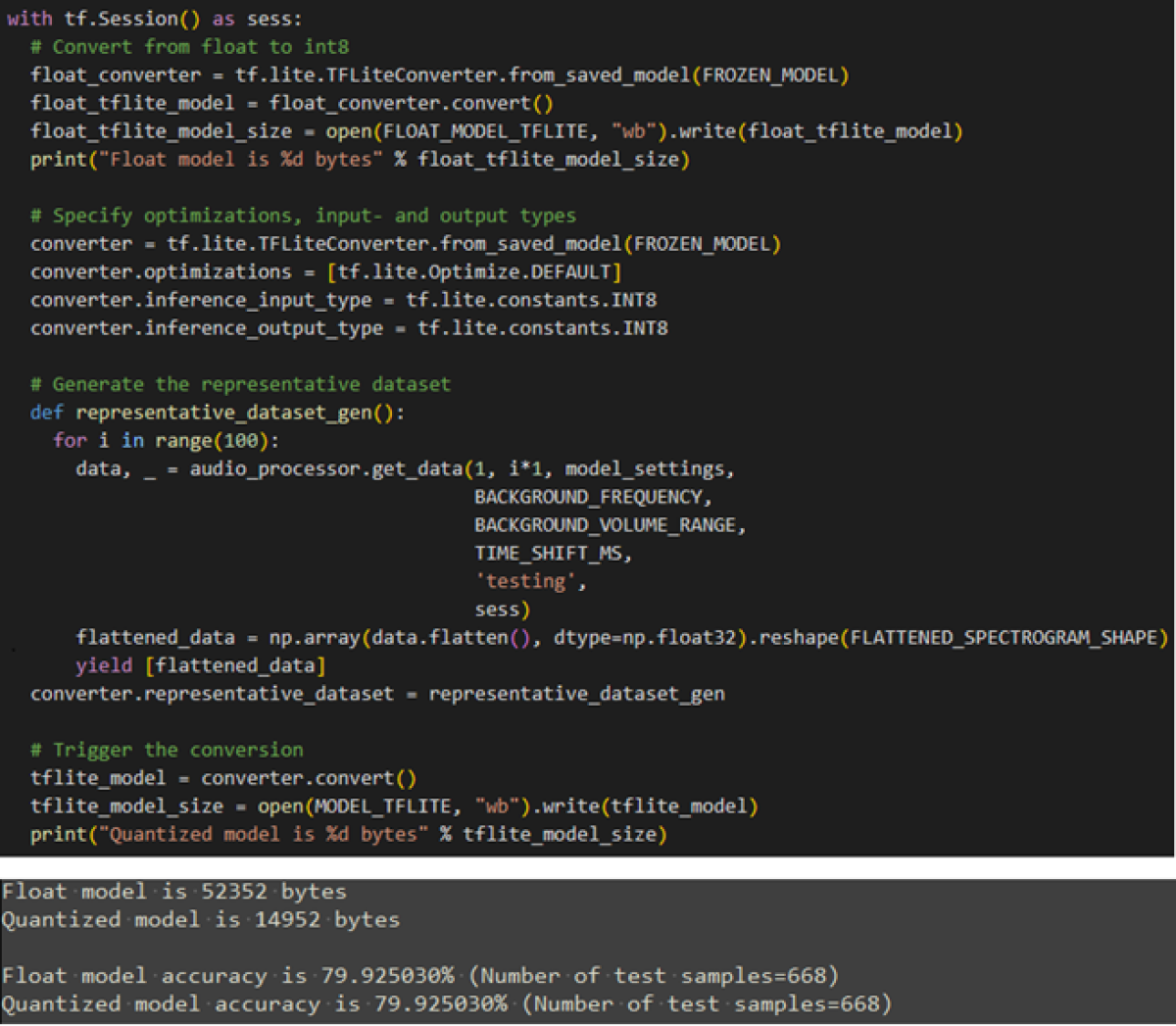
As shown in the output above, the conversion did not cause any loss in accuracy.
4.2 From TensorFlow Lite to TensorFlow Lite Micro
We’ve now reached the final stage of the TensorFlow framework.
The goal is to generate a model that can run inference directly on the hardware. This is handled by TensorFlow (TF) Lite Micro.
Here we push compression to the limit by removing all functionalities that are not strictly necessary. TF Lite Micro is purpose-built for embedded systems. For example, it allocates no dynamic memory, requires no file system, and avoids standard library functions.
As a result, TF Lite Micro is highly portable across different platforms.
The following subchapters describe how TF Lite Micro is used.
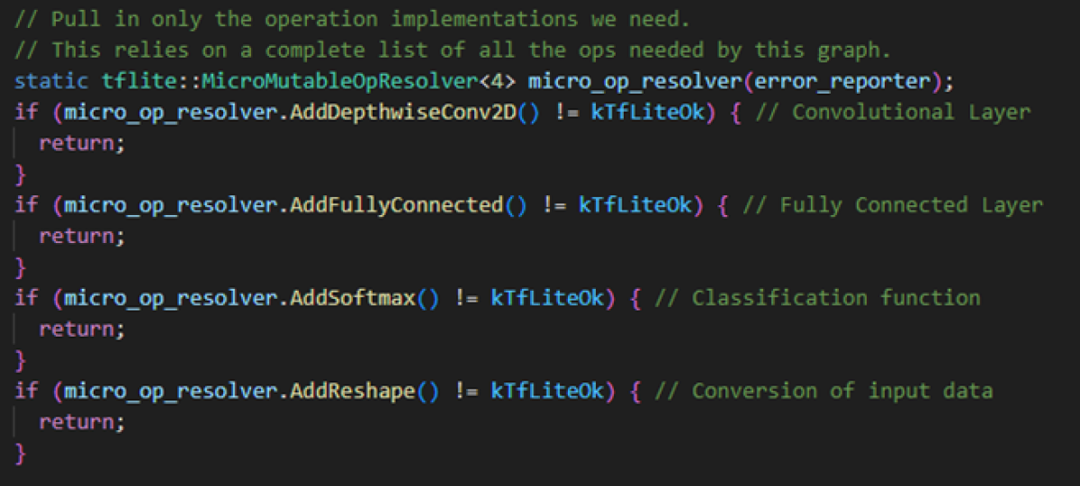
4.2.1 OpResolver
The Operation Resolver specifies which functions of the TensorFlow library should be used and which not. This depends on the layer types and the functions they need for input processing or classification.
In our case, the required functions are:
4.2.2 Interpreter
In software, interpreting means executing a program by following a data structure in memory.
In contrast, compiled execution defines the program's behavior at compile time.
On embedded devices, we typically prefer compiled code because a single line of code translates into just 3–4 processor instructions. If interpreted, the same line would first need to be passed to an interpreter, which would then translate it – resulting in more overhead than the executable code itself.
With AI models, the situation is different. Every model invocation generates thousands of instructions, so the overhead from interpretation is negligible. It makes no difference whether the model is compiled or interpreted.
The interpreter offers important benefits: for instance, the model can be swapped without recompiling the code – enabling shorter iteration cycles if the model is refined.
Furthermore, the same operator code can be reused across different models in the system.
In the end, this allows for the same model to be deployed in various systems.
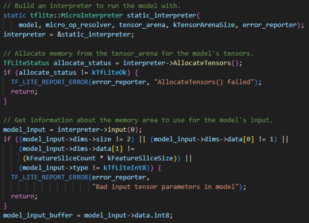
In the code above, you can see that the interpreter requires the model, the OpResolver, and a TensorArena to be passed to it.
The TensorArena is a dedicated memory area that the interpreter uses for input, output, and intermediate steps, since dynamic memory allocation is avoided.
The size depends on the model used and must be adjusted accordingly.
4.2.3 FlatBuffer
The model itself is stored in a FlatBuffer. A FlatBuffer is an array of bytes that contains the operations and weights of the model. Additionally, metadata such as version, quantization level, or parameters are stored in it.
The format in which this array is read is defined in a schema file. This specifies where certain elements can be found in the data structure. The compiler generates code from this to access these elements in the correct way.
The FlatBuffer is not stored in the TensorArena, but in a read-only area, typically in flash memory, since our model cannot change at runtime.
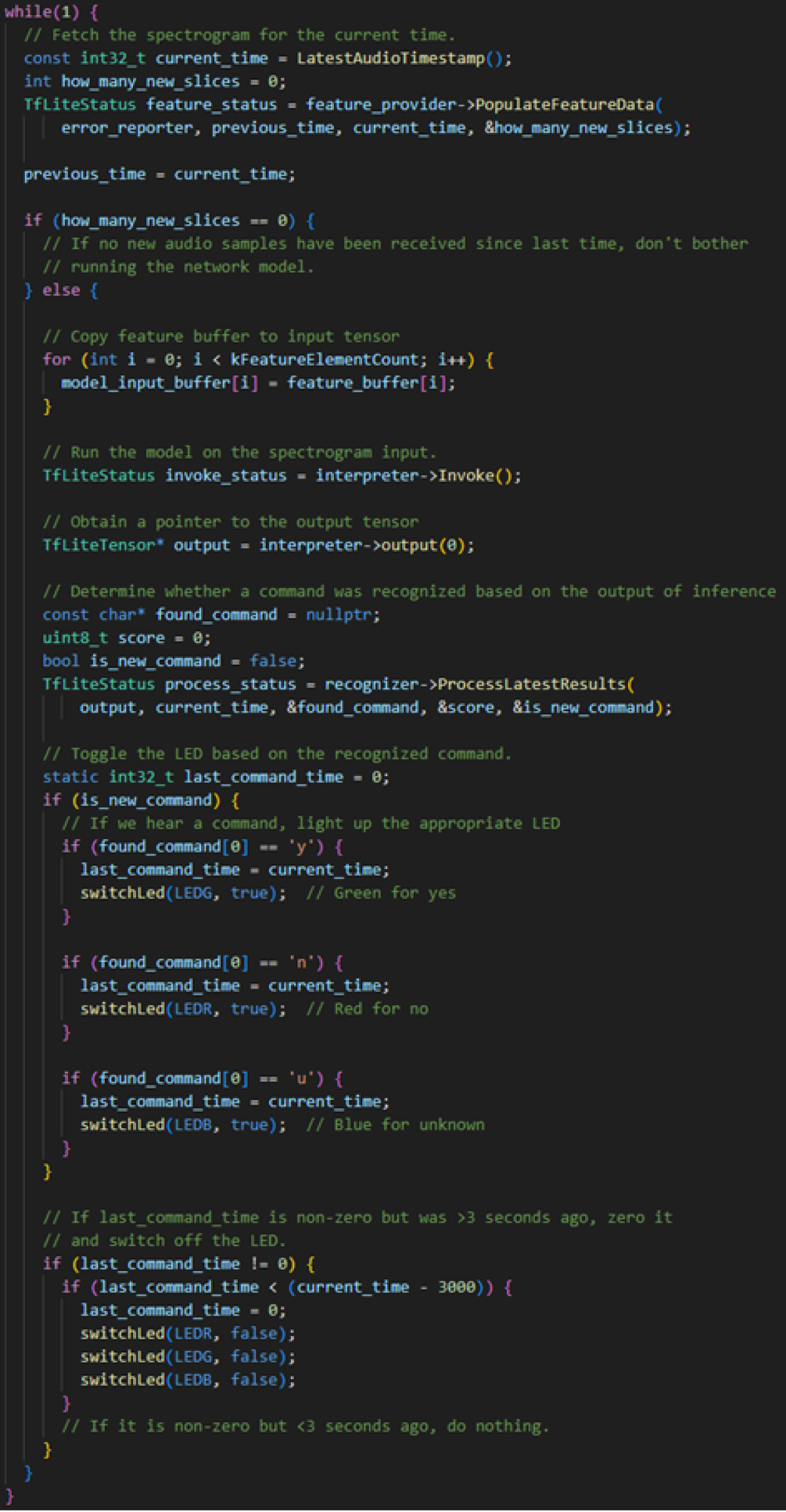
Implementation and result
Some code still needs to be written to run the AI model on the embedded device. This includes reading data from the microphone, passing this data to the model, evaluating the results, and finally controlling the LED in the corresponding color.
The "sliding window" approach is used for reading and further processing the microphone signals. In this method, audio signals are continuously grouped into 1-second segments and passed to the neural network.
Sliding Window Approach
Source Code "Keyword Spotting" Application
This video shows that the device functions as initially specified.
Click here to watch the video.
Conclusion
As mentioned in the previous post about AI, artificial intelligence has arrived in embedded systems and opens up numerous new application possibilities.
For our example, we used a conventional microcontroller. However, there are now chips on the market with dedicated AI accelerators and specialized hardware. Our example demonstrates that these are not necessarily required to implement a functional AI project.
We understand this technology and are excited to see what exciting projects and application areas can be realized in the embedded world in the future.
With our know-how, we actively shape this future and are happy to support you in your next development.

Mathieu Bourquin
BSc in Electrical and Communication Engineering, Bern University of Applied Sciences
Embedded Software Engineer
About the author
Mathieu Bourquin has been working as an Embedded Software Engineer at CSA for four years.
He supports clients in the medical technology sector and is a specialist in developing firmware in C/C++ and implementing functional safety. His interest in new technologies and his motivation for continuous learning have inevitably led him to AI technology.